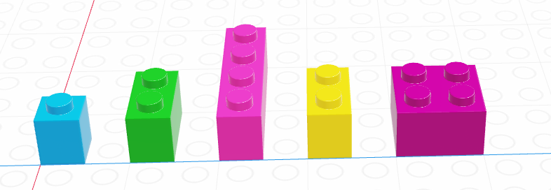
[1] TRUE FALSE FALSE FALSEx | y # OR[1] TRUE TRUE TRUE FALSE!x & y # NOT X AND Y[1] FALSE TRUE FALSE FALSEx & !y # X AND NOT Y[1] FALSE FALSE TRUE FALSEReading: 25 minute(s) at 200 WPM.
Videos: 28 minutes
A prerequisite for this course is an introductory programming course. Therefore, there is some assumed knowledge. Maybe you have not seen these concepts in R, but you have already developed a base for logically thinking through a computing problem in another language.
This chapter is meant to provide a resource for the basics of programming (in R) and gives me a place to refer back to (as need be) in future chapters.
In this chapter you will:
R.R.It is helpful when teaching a topic as technical as programming to ensure that everyone starts from the same basic foundational understanding and mental model of how things work. When teaching geology, for instance, the instructor should probably make sure that everyone understands that the earth is a round ball and not a flat plate – it will save everyone some time later.
We all use computers daily - we carry them around with us on our wrists, in our pockets, and in our backpacks. This is no guarantee, however, that we understand how they work or what makes them go.
Here is a short 3-minute video on the basic hardware that makes up your computer. It is focused on desktops, but the same components (with the exception of the optical drive) are commonly found in cell phones, smart watches, and laptops.
When programming, it is usually helpful to understand the distinction between RAM and disk storage (hard drives). We also need to know at least a little bit about processors (so that we know when we’ve asked our processor to do too much). Most of the other details aren’t necessary (for now).
Operating systems, such as Windows, MacOS, or Linux, are a sophisticated program that allows CPUs to keep track of multiple programs and tasks and execute them at the same time.
Evidently, there has been a bit of generational shift as computers have evolved: the “file system” metaphor itself is outdated because no one uses physical files anymore. This article is an interesting discussion of the problem: it makes the argument that with modern search capabilities, most people use their computers as a laundry hamper instead of as a nice, organized filing cabinet.
Regardless of how you tend to organize your personal files, it is probably helpful to understand the basics of what is meant by a computer file system – a way to organize data stored on a hard drive. Since data is always stored as 0’s and 1’s, it’s important to have some way to figure out what type of data is stored in a specific location, and how to interpret it.
Stop watching at 4:16.
That’s not enough, though - we also need to know how computers remember the location of what is stored where. Specifically, we need to understand file paths.
Recommend watching - helpful for understanding file paths!
When you write a program, you may have to reference external files - data stored in a .csv file, for instance, or a picture. Best practice is to create a file structure that contains everything you need to run your entire project in a single file folder (you can, and sometimes should, have sub-folders).
For now, it is enough to know how to find files using file paths, and how to refer to a file using a relative file path from your base folder. In this situation, your “base folder” is known as your working directory - the place your program thinks of as home.
In Chapter 1, we will discuss Directories, Paths, and Projects as they relate to R and getting setup to be successful in this course.
This section introduces some of the most important tools for working with data: vectors, matrices, loops, and if statements. It would be nice to gradually introduce each one of these topics separately, but they tend to go together, especially when you’re talking about programming in the context of data processing.
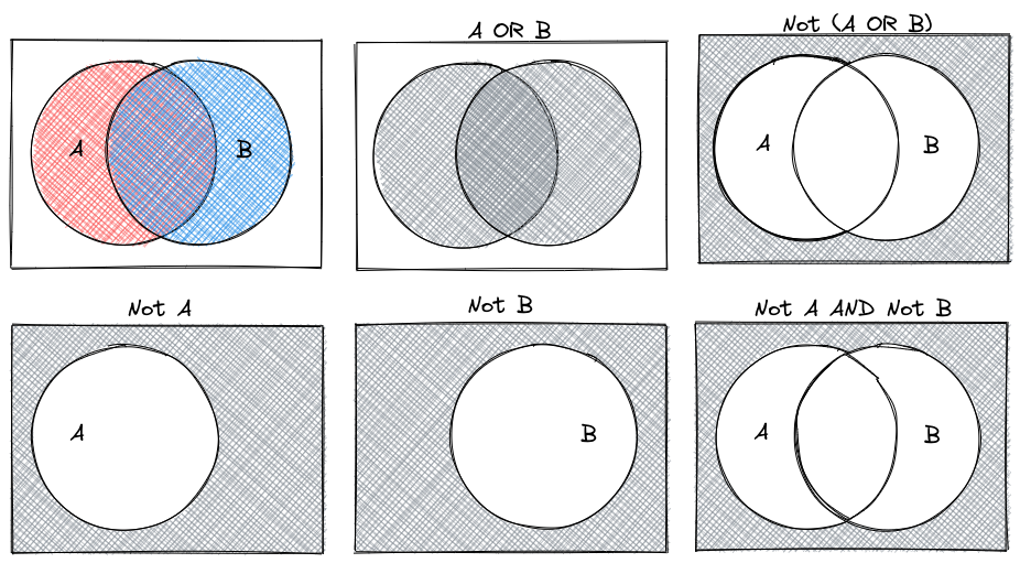
Before we start talking about data structures and control structures, though, we’re going to take a minute to review some concepts from mathematical logic. This will be useful for both data structures and control structures, so stick with me for a few minutes.
We can combine logical statements using and, or, and not.
In R, we use ! to symbolize NOT.
Order of operations dictates that NOT is applied before other operations. So NOT X AND Y is read as (NOT X) AND (Y). You must use parentheses to change the way this is interpreted.
De Morgan’s Laws are a set of rules for how to combine logical statements. You can represent them in a number of ways:
 Suppose that we set the convention that
 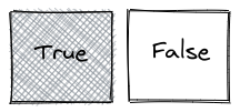 .
.
While we will discuss data types more in depth during class, it is important to have a base grasp on the types of data you might see in a programming language.
Let’s start this section with some basic vocabulary.
1, 2, "Hello, World", and so on.2 is an integer, "Hello, World" is a string (it contains a “string” of letters). Strings are in quotation marks to let us know that they are not variable names.In R, there are some very basic data types:
logical or boolean - FALSE/TRUE or 0/1 values. Sometimes, boolean is shortened to bool
integer - whole numbers (positive or negative)
double or float or numeric- decimal numbers.
R uses the name numeric to indicate a decimal value, regardless of precision.character or string - holds text, usually enclosed in quotes.
If you don’t know what type a value is, R has a function to help you with that.
class(FALSE)
class(2L) # by default, R treats all numbers as numeric/decimal values.
          # The L indicates that we're talking about an integer.
class(2)
class("Hello, programmer!")
[1] "logical"
[1] "integer"
[1] "numeric"
[1] "character"In R, boolean values are TRUE and FALSE. Capitalization matters a LOT.
Other things matter too: if we try to write a million, we would write it 1000000 instead of 1,000,000. Commas are used for separating numbers, not for proper spacing and punctuation of numbers. This is a hard thing to get used to but very important – especially when we start reading in data.
Programming languages use variables - names that refer to values. Think of a variable as a container that holds something - instead of referring to the value, you can refer to the container and you will get whatever is stored inside.
In R, we assign variables values using the syntax object_name <- value You can read this as “object name gets value” in your head.
message <- "So long and thanks for all the fish"
year <- 2025
the_answer <- 42L
earth_demolished <- FALSE
Note that in R, we assign variables values using the <- operator. Technically, = will work for assignment, but <- is more common than = in R by convention.
We can then use the variables - do numerical computations, evaluate whether a proposition is true or false, and even manipulate the content of strings, all by referencing the variable by name.
There are only two hard things in Computer Science: cache invalidation and naming things.
– Phil Karlton
Object names must start with a letter and can only contain letters, numbers, _, and . in R.
What happens if we try to create a variable name that isn’t valid?
Starting a variable name with a number will get you an error message that lets you know that something isn’t right - “unexpected symbol”.
1st_thing <- "check your variable names!"Error: <text>:1:2: unexpected symbol
1: 1st_thing
^Naming things is difficult! When you name variables, try to make the names descriptive - what does the variable hold? What are you going to do with it? The more (concise) information you can pack into your variable names, the more readable your code will be.
Why is naming things hard? - Blog post by Neil Kakkar
There are a few different conventions for naming things that may be useful:
some_people_use_snake_case, where words are separated by underscoressomePeopleUseCamelCase, where words are appended but anything after the first word is capitalized (leading to words with humps like a camel).some.people.use.periodsvariables_thatLookLike.this and they are almost universally hated.As long as you pick ONE naming convention and don’t mix-and-match, you’ll be fine. It will be easier to remember what you named your variables (or at least guess) and you’ll have fewer moments where you have to go scrolling through your script file looking for a variable you named.
We talked about values and types above, but skipped over a few details because we didn’t know enough about variables. It’s now time to come back to those details.
What happens when we have an integer and a numeric type and we add them together? Hopefully, you don’t have to think too hard about what the result of 2 + 3.5 is, but this is a bit more complicated for a computer for two reasons: storage, and arithmetic.
In days of yore, programmers had to deal with memory allocation - when declaring a variable, the programmer had to explicitly define what type the variable was. This tended to look something like the code chunk below:
int a = 1
double b = 3.14159
Typically, an integer would take up 32 bits of memory, and a double would take up 64 bits, so doubles used 2x the memory that integers did. R is dynamically typed, which means you don’t have to deal with any of the trouble of declaring what your variables will hold - the computer automatically figures out how much memory to use when you run the code. So we can avoid the discussion of memory allocation and types because we’re using higher-level languages that handle that stuff for us2.
But the discussion of types isn’t something we can completely avoid, because we still have to figure out what to do when we do operations on things of two different types - even if memory isn’t a concern, we still have to figure out the arithmetic question.
So let’s see what happens with a couple of examples, just to get a feel for type conversion (aka type casting or type coercion), which is the process of changing an expression from one data type to another.
mode(2L + 3.14159) # add integer 2 and pi[1] "numeric"mode(2L + TRUE) # add integer 2 and TRUE[1] "numeric"mode(TRUE + FALSE) # add TRUE and FALSE[1] "numeric"All of the examples above are ‘numeric’ - basically, a catch-all class for things that are in some way, shape, or form numbers. Integers and decimal numbers are both numeric, but so are logicals (because they can be represented as 0 or 1).
You may be asking yourself at this point why this matters, and that’s a decent question. We will eventually be reading in data from spreadsheets and other similar tabular data, and types become very important at that point, because we’ll have to know how R handles type conversions.
Do a bit of experimentation - what happens when you try to add a string and a number? Which types are automatically converted to other types? Fill in the following table in your notes:
Adding a ___ and a ___ produces a ___:
| Logical | Integer | Decimal | String | |
|---|---|---|---|---|
| Logical | ||||
| Integer | ||||
| Decimal | ||||
| String |
Above, we looked at automatic type conversions, but in many cases, we also may want to convert variables manually, specifying exactly what type we’d like them to be. A common application for this in data analysis is when there are “*” or “.” or other indicators in an otherwise numeric column of a spreadsheet that indicate missing data: when this data is read in, the whole column is usually read in as character data. So we need to know how to tell R that we want our string to be treated as a number, or vice-versa.
In R, we can explicitly convert a variable’s type using as.XXX() functions, where XXX is the type you want to convert to (as.numeric, as.integer, as.logical, as.character, etc.).
x <- 3
y <- "3.14159"

x + y
Error in x + y: non-numeric argument to binary operatorx + as.numeric(y)[1] 6.14159In addition to variables, functions are extremely important in programming.
Let’s first start with a special class of functions called operators. You’re probably familiar with operators as in arithmetic expressions: +, -, /, *, and so on.
Here are a few of the most important ones:
| Operation | R symbol |
|---|---|
| Addition | + |
| Subtraction | - |
| Multiplication | * |
| Division | / |
| Integer Division | %/% |
| Modular Division | %% |
| Exponentiation | ^ |
Note that integer division is the whole number answer to A/B, and modular division is the fractional remainder when A/B.
So 14 %/% 3 would be 4, and 14 %% 3 would be 2.
Note that these operands are all intended for scalar operations (operations on a single number) - vectorized versions, such as matrix multiplication, are somewhat more complicated.
R operates under the same mathematical rules of precedence that you learned in school. You may have learned the acronym PEMDAS, which stands for Parentheses, Exponents, Multiplication/Division, and Addition/Subtraction. That is, when examining a set of mathematical operations, we evaluate parentheses first, then exponents, and then we do multiplication/division, and finally, we add and subtract.
(1+1)^(5-2) # 2 ^ 3 = 8[1] 81 + 2^3 * 4 # 1 + (8 * 4)[1] 333*1^3 # 3 * 1[1] 3You will have to use functions to perform operations on strings, as R does not have string operators. In R, to concatenate things, we need to use functions: paste or paste0:
paste("first", "second", sep = " ")[1] "first second"paste("first", "second", collapse = " ")[1] "first second"[1] "first" "second"[1] "first second"[1] "a-first b-second c-third d-fourth"# sep is used to collapse parameters, then collapse is used to collapse vectors
paste0(c("a", "b", "c"))[1] "a" "b" "c"paste0("a", "b", "c") # equivalent to paste(..., sep = "")[1] "abc"You don’t need to understand the details of this at this point in the class, but it is useful to know how to combine strings.
Functions are sets of instructions that take arguments and return values. Strictly speaking, operators (like those above) are a special type of functions – but we aren’t going to get into that now.
We’re also not going to talk about how to create our own functions just yet. Instead, I’m going to show you how to use functions.
It may be helpful at this point to print out the R reference card3. This cheat sheet contains useful functions for a variety of tasks.
Methods are a special type of function that operate on a specific variable type. In R, you would get the length of a string variable using length(my_string).
Right now, it is not really necessary to know too much more about functions than this: you can invoke a function by passing in arguments, and the function will do a task and return the value.
In the previous section, we discussed 4 different data types: strings/characters, numeric/double/floats, integers, and logical/booleans. As you might imagine, things are about to get more complicated.
Data structures are more complicated arrangements of information.
| Homogeneous | Heterogeneous | |
|---|---|---|
| 1D | vector | list |
| 2D | matrix | data frame |
| N-D | array |
A list is a one-dimensional column of heterogeneous data - the things stored in a list can be of different types.
x <- list("a", 3, FALSE)
x
[[1]]
[1] "a"
[[2]]
[1] 3
[[3]]
[1] FALSEThe most important thing to know about lists, for the moment, is how to pull things out of the list. We call that process indexing.
Every element in a list has an index (a location, indicated by an integer position)4.
In R, we count from 1.
x <- list("a", 3, FALSE)

x[1] # This returns a list
[[1]]
[1] "a"x[1:2] # This returns multiple elements in the list[[1]]
[1] "a"
[[2]]
[1] 3x[[1]] # This returns the item[1] "a"x[[1:2]] # This doesn't work - you can only use [[]] with a single indexError in x[[1:2]]: subscript out of boundsList indexing with [] will return a list with the specified elements.
To actually retrieve the item in the list, use [[]]. The only downside to [[]] is that you can only access one thing at a time.
We’ll talk more about indexing as it relates to vectors, but indexing is a general concept that applies to just about any multi-value object.
A vector is a one-dimensional column of homogeneous data. Homogeneous means that every element in a vector has the same data type.
We can have vectors of any data type and length we want: 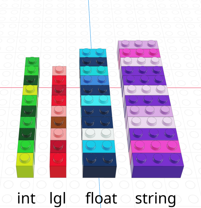
Each element in a vector has an index - an integer telling you what the item’s position within the vector is. I’m going to demonstrate indices with the string vector
| R | |
|---|---|
| 1-indexed language | |
| Count elements as 1, 2, 3, 4, …, N | |
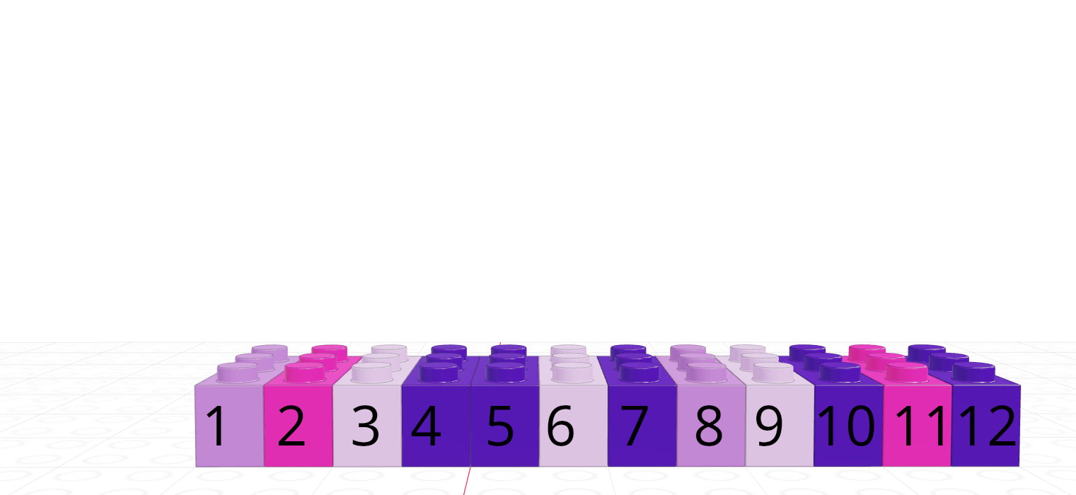 |
In R, we create vectors with the c() function, which stands for “concatenate” - basically, we stick a bunch of objects into a row.
digits_pi <- c(3, 1, 4, 1, 5, 9, 2, 6, 5, 3, 5)

# Access individual entries
digits_pi[1]
[1] 3digits_pi[2][1] 1digits_pi[3][1] 4# R is 1-indexed - a list of 11 things goes from 1 to 11
digits_pi[0]numeric(0)digits_pi[11][1] 5# Print out the vector
digits_pi [1] 3 1 4 1 5 9 2 6 5 3 5We can pull out items in a vector by indexing, but we can also replace specific things as well:
favorite_cats <- c("Grumpy", "Garfield", "Jorts", "Jean")

favorite_cats
[1] "Grumpy" "Garfield" "Jorts" "Jean" favorite_cats[2] <- "Nyan Cat"
favorite_cats[1] "Grumpy" "Nyan Cat" "Jorts" "Jean" If you’re curious about any of these cats, see the footnotes5.
As you might imagine, we can create vectors of all sorts of different data types. One particularly useful trick is to create a logical vector that goes along with a vector of another type to use as a logical index.
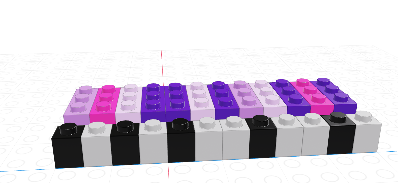
If we let the black lego represent “True” and the grey lego represent “False”, we can use the logical vector to pull out all values in the main vector.
| Black = True, Grey = False | Grey = True, Black = False |
|---|---|
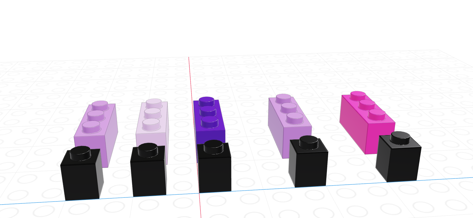 |
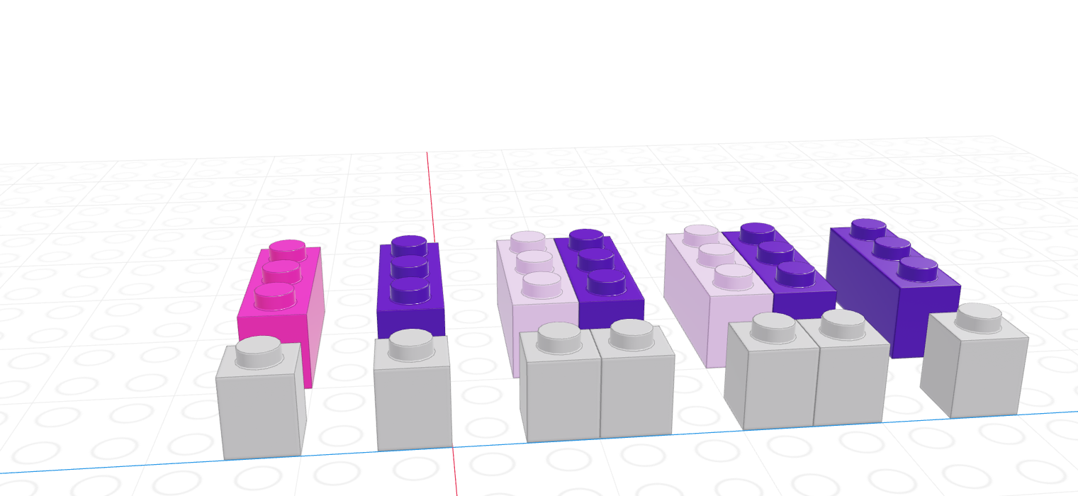 |
Note that for logical indexing to work properly, the logical index must be the same length as the vector we’re indexing. This constraint will return when we talk about data frames, but for now just keep in mind that logical indexing doesn’t make sense when this constraint isn’t true.
# Define a character vector
weekdays <- c("Sunday", "Monday", "Tuesday", "Wednesday", "Thursday", "Friday", "Saturday")
weekend <- c("Sunday", "Saturday")

# Create logical vectors
relax_days <- c(1, 0, 0, 0, 0, 0, 1) # doing this the manual way
relax_days <- weekdays %in% weekend # This creates a logical vector
                                    # with less manual construction
relax_days
[1] TRUE FALSE FALSE FALSE FALSE FALSE TRUEschool_days <- !relax_days # FALSE if weekend, TRUE if not
school_days[1] FALSE TRUE TRUE TRUE TRUE TRUE FALSE# Using logical vectors to index the character vector
weekdays[school_days] # print out all school days[1] "Monday" "Tuesday" "Wednesday" "Thursday" "Friday" As vectors are a collection of things of a single type, what happens if we try to make a vector with differently-typed things?
c(2L, FALSE, 3.1415, "animal") # all converted to strings[1] "2" "FALSE" "3.1415" "animal"c(2L, FALSE, 3.1415) # converted to numerics[1] 2.0000 0.0000 3.1415c(2L, FALSE) # converted to integers[1] 2 0As a reminder, this is an example of implicit type conversion - R decides what type to use for you, going with the type that doesn’t lose data but takes up as little space as possible.
A matrix is the next step after a vector - it’s a set of values arranged in a two-dimensional, rectangular format.
# Minimal matrix in R: take a vector,
# tell R how many rows you want
matrix(1:12, nrow = 3)
[,1] [,2] [,3] [,4]
[1,] 1 4 7 10
[2,] 2 5 8 11
[3,] 3 6 9 12matrix(1:12, ncol = 3) # or columns [,1] [,2] [,3]
[1,] 1 5 9
[2,] 2 6 10
[3,] 3 7 11
[4,] 4 8 12# by default, R will fill in column-by-column
# the byrow parameter tells R to go row-by-row
matrix(1:12, nrow = 3, byrow = T) [,1] [,2] [,3] [,4]
[1,] 1 2 3 4
[2,] 5 6 7 8
[3,] 9 10 11 12# We can also easily create square matrices
# with a specific diagonal (this is useful for modeling)
diag(rep(1, times = 4)) [,1] [,2] [,3] [,4]
[1,] 1 0 0 0
[2,] 0 1 0 0
[3,] 0 0 1 0
[4,] 0 0 0 1Most of the problems we’re going to work on will not require much in the way of matrix or array operations. For now, you need the following:
R uses [row, column] to index matrices. To extract the bottom-left element of a 3x4 matrix, we would use [3,1] to get to the third row and first column entry; in python, we would use [2,0] (remember that Python is 0-indexed).
As with vectors, you can replace elements in a matrix using assignment.
my_mat <- matrix(1:12, nrow = 3, byrow = T)

my_mat[3,1] <- 500

my_mat
[,1] [,2] [,3] [,4]
[1,] 1 2 3 4
[2,] 5 6 7 8
[3,] 500 10 11 12There are a number of matrix operations that we need to know for basic programming purposes:
x <- matrix(c(1, 2, 3, 4), nrow = 2, byrow = T)
y <- matrix(c(5, 6), nrow = 2)

# Scalar multiplication
x * 3
[,1] [,2]
[1,] 3 6
[2,] 9 123 * x [,1] [,2]
[1,] 3 6
[2,] 9 12# Transpose
t(x) [,1] [,2]
[1,] 1 3
[2,] 2 4t(y) [,1] [,2]
[1,] 5 6# matrix multiplication (dot product)
x %*% y [,1]
[1,] 17
[2,] 39Arrays are a generalized n-dimensional version of a vector: all elements have the same type, and they are indexed using square brackets in both R and python: [dim1, dim2, dim3, ...]
I don’t think you will need to create 3+ dimensional arrays in this class, but if you want to try it out, here is some code.
Note that displaying this requires 2 slices, since it’s hard to display 3D information in a 2D terminal arrangement.
The focus of this course is more on working with data - however in prior programming courses you have likely developed the logical thinking to work with Control structures. Control structures are statements in a program that determine when code is evaluated (and how many times it might be evaluated). There are two main types of control structures: if-statements and loops.
Before we start on the types of control structures, let’s get in the right mindset. We’re all used to “if-then” logic, and use it in everyday conversation, but computers require another level of specificity when you’re trying to provide instructions.
Check out this video of the classic “make a peanut butter sandwich instructions challenge”:
Here’s another example:

The key takeaways from these bits of media are that you should read this section with a focus on exact precision - state exactly what you mean, and the computer will do what you say. If you instead expect the computer to get what you mean, you’re going to have a bad time.
Conditional statements determine if code is evaluated.
They look like this:
if (condition)
  then
    (thing to do)
  else
    (other thing to do)
The else (other thing to do) part may be omitted.
When this statement is read by the computer, the computer checks to see if condition is true or false. If the condition is true, then (thing to do) is also run. If the condition is false, then (other thing to do) is run instead.
[1] "x = 3 ; y = 8"The logical condition after if must be in parentheses. It is common to then enclose the statement to be run if the condition is true in {} so that it is clear what code matches the if statement. You can technically put the condition on the line after the if (x > 2) line, and everything will still work, but then it gets hard to figure out what to do with the else statement - it technically would also go on the same line, and that gets hard to read.
So while the 2nd version of the code technically works, the first version with the brackets is much easier to read and understand. Please try to emulate the first version!
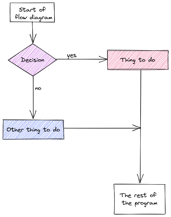
A common way to represent conditional logic is to draw a flow chart diagram.
In a flow chart, conditional statements are represented as diamonds, and other code is represented as a rectangle. Yes/no or True/False branches are labeled. Typically, after a conditional statement, the program flow returns to a single point.
The US Tax code has brackets, such that the first $10,275 of your income is taxed at 10%, anything between $10,275 and $41,775 is taxed at 12%, and so on.
Here is the table of tax brackets for single filers in 2022:
| rate | Income |
|---|---|
| 10% | $0 to $10,275 |
| 12% | $10,275 to $41,775 |
| 22% | $41,775 to $89,075 |
| 24% | $89,075 to $170,050 |
| 32% | $170,050 to $215,950 |
| 35% | $215,950 to $539,900 |
| 37% | $539,900 or more |
Note: For the purposes of this problem, we’re ignoring the personal exemption and the standard deduction, so we’re already simplifying the tax code.
Write a set of if statements that assess someone’s income and determine what their overall tax rate is.
Hint: You may want to keep track of how much of the income has already been taxed in a variable and what the total tax accumulation is in another variable.
# Start with total income
income <- 200000

# x will hold income that hasn't been taxed yet
x <- income
# y will hold taxes paid
y <- 0

if (x <= 10275) {
  y <- x*.1 # tax paid
  x <- 0 # All money has been taxed
} else {
  y <- y + 10275 * .1
  x <- x - 10275 # Money remaining that hasn't been taxed
}

if (x <= (41775 - 10275)) {
  y <- y + x * .12
  x <- 0
} else {
  y <- y + (41775 - 10275) * .12
  x <- x - (41775 - 10275)
}

if (x <= (89075 - 41775)) {
  y <- y + x * .22
  x <- 0
} else {
  y <- y + (89075 - 41775) * .22
  x <- x - (89075 - 41775)
}

if (x <= (170050 - 89075)) {
  y <- y + x * .24
  x <- 0
} else {
  y <- y + (170050 - 89075) * .24
  x <- x - (170050 - 89075)
}

if (x <= (215950 - 170050)) {
  y <- y + x * .32
  x <- 0
} else {
  y <- y + (215950 - 170050) * .32
  x <- x - (215950 - 170050)
}

if (x <= (539900 - 215950)) {
  y <- y + x * .35
  x <- 0
} else {
  y <- y + (539900 - 215950) * .35
  x <- x - (539900 - 215950)
}

if (x > 0) {
  y <- y + x * .37
}


print(paste("Total Tax Rate on $", income, " in income = ", round(y/income, 4)*100, "%"))
[1] "Total Tax Rate on $ 2e+05 in income = 22.12 %"Let’s explore using program flow maps for a slightly more complicated problem: The tax bracket example that we used to demonstrate if statement syntax.
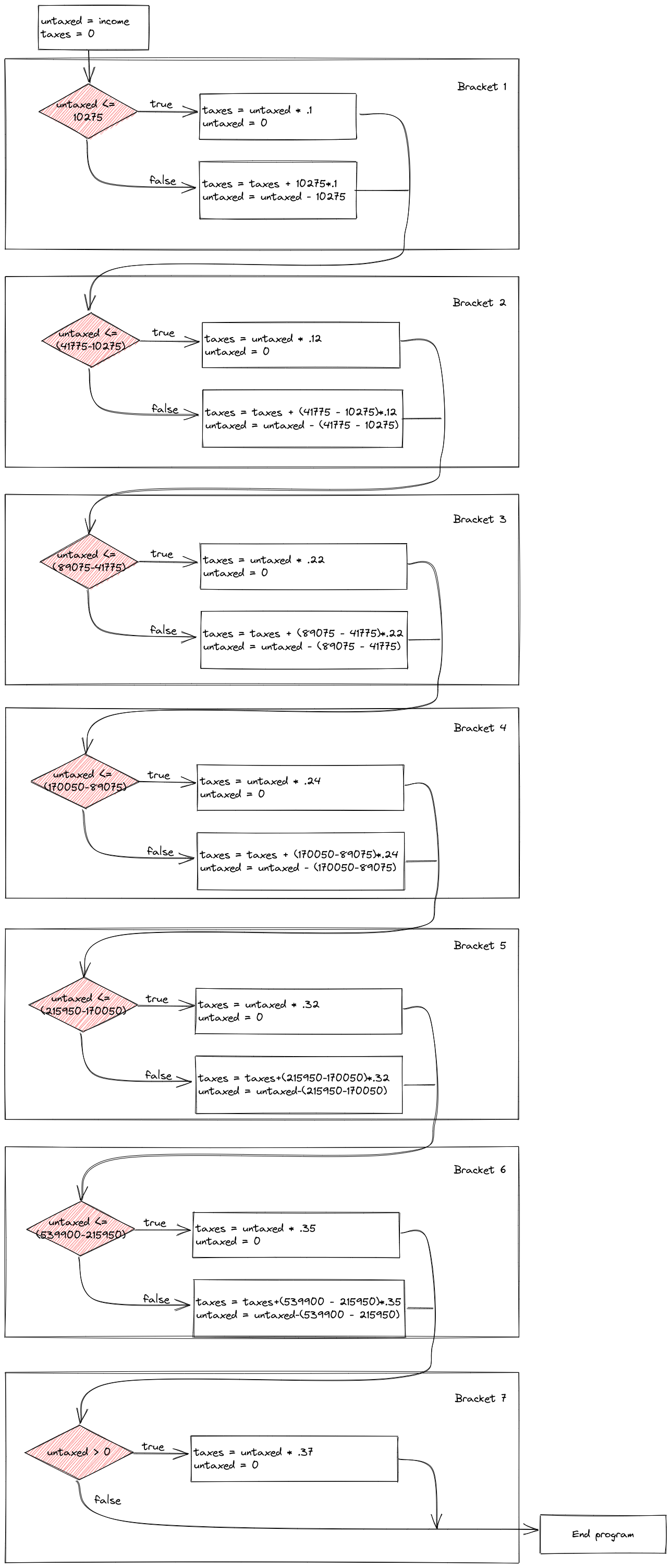
Control flow diagrams can be extremely helpful when figuring out how programs work (and where gaps in your logic are when you’re debugging). It can be very helpful to map out your program flow as you’re untangling a problem.
In many cases, it can be helpful to have a long chain of conditional statements describing a sequence of alternative statements.
For instance, suppose I want to determine what categorical age bracket someone falls into based on their numerical age. All of the bins are mutually exclusive - you can’t be in the 25-40 bracket and the 41-55 bracket.
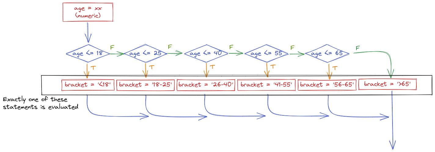
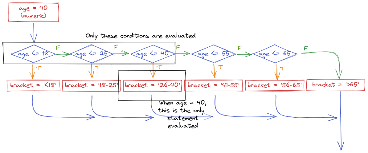
The important thing to realize when examining this program flow map is that if age <= 18 is true, then none of the other conditional statements even get evaluated. That is, once a statement is true, none of the other statements matter. Because of this, it is important to place the most restrictive statement first.
If for some reason you wrote your conditional statements in the wrong order, the wrong label would get assigned:
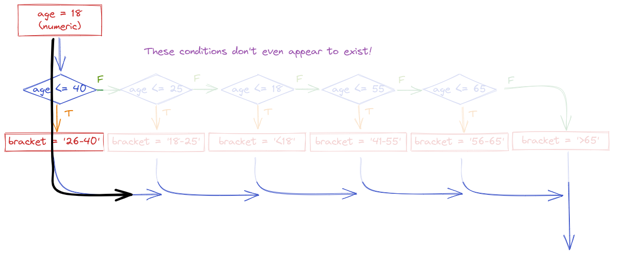
In code, we would write this statement using else-if (or elif) statements.
age <- 40 # change this as you will to see how the code works

if (age < 18) {
  bracket <- "<18"
} else if (age <= 25) {
  bracket <- "18-25"
} else if (age <= 40) {
  bracket <- "26-40"
} else if (age <= 55) {
  bracket <- "41-55"
} else if (age <= 65) {
  bracket <- "56-65"
} else {
  bracket <- ">65"
}

bracket
[1] "26-40"Often, we write programs which update a variable in a way that the new value of the variable depends on the old value:
x = x + 1This means that we add one to the current value of x.
Before we write a statement like this, we have to initialize the value of x because otherwise, we don’t know what value to add one to.
x = 0
x = x + 1
We sometimes use the word increment to talk about adding one to the value of x; decrement means subtracting one from the value of x.
A particularly powerful tool for making these types of repetitive changes in programming is the loop, which executes statements a certain number of times. Loops can be written in several different ways, but all loops allow for executing a block of code a variable number of times.
We just discussed conditional statements, where a block of code is only executed if a logical statement is true.
The simplest type of loop is the while loop, which executes a block of code until a statement is no longer true.
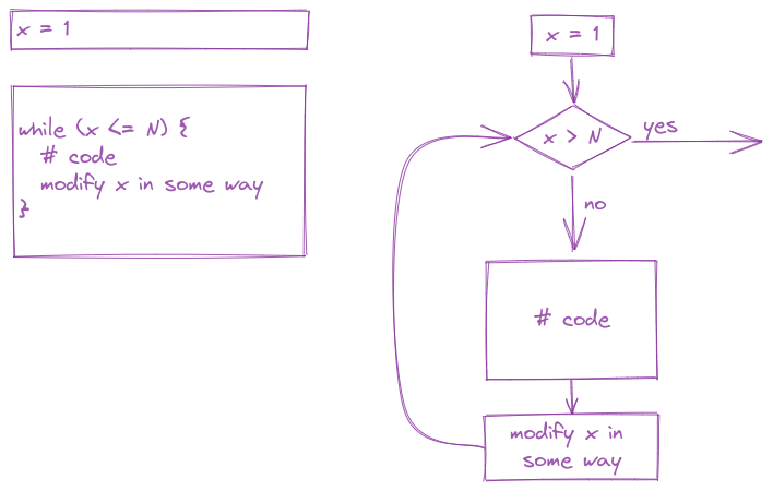
x <- 0

while (x < 10) {
  # Everything in here is executed
  # during each iteration of the loop
  print(x)
  x <- x + 1
}
[1] 0
[1] 1
[1] 2
[1] 3
[1] 4
[1] 5
[1] 6
[1] 7
[1] 8
[1] 9Write a while loop that verifies that \[\lim_{N \rightarrow \infty} \prod_{k=1}^N \left(1 + \frac{1}{k^2}\right) = \frac{e^\pi - e^{-\pi}}{2\pi}.\]
Terminate your loop when you get within 0.0001 of \(\frac{e^\pi - e^{-\pi}}{2\pi}\). At what value of \(k\) is this point reached?
Breaking down math notation for code:
If you are unfamiliar with the notation \(\prod_{k=1}^N f(k)\), this is the product of \(f(k)\) for \(k = 1, 2, ..., N\), \[f(1)\cdot f(2)\cdot ... \cdot f(N)\]
To evaluate a limit, we just keep increasing \(N\) until we get arbitrarily close to the right hand side of the equation.
In this problem, we can just keep increasing \(k\) and keep track of the cumulative product. So we define k=1, prod = 1, and ans before the loop starts. Then, we loop over k, multiplying prod by \((1 + 1/k^2)\) and then incrementing \(k\) by one each time. At each iteration, we test whether prod is close enough to ans to stop the loop.
Another common type of loop is a for loop. In a for loop, we run the block of code, iterating through a series of values (commonly, one to N, but not always). Generally speaking, for loops are known as definite loops because the code inside a for loop is executed a specific number of times. While loops are known as indefinite loops because the code within a while loop is evaluated until the condition is falsified, which is not always a known number of times.
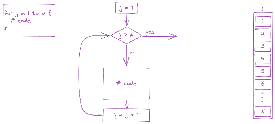
for (i in 1:5 ) {
  print(i)
}
[1] 1
[1] 2
[1] 3
[1] 4
[1] 5For loops are often run from 1 to N but in essence, a for loop is run for every value of a vector (which is why loops are included in the same chapter as vectors).
For instance, in R, there is a built-in variable called month.name. Type month.name into your R console to see what it looks like. If we want to iterate along the values of month.name, we can:
for (i in month.name)
  print(i)
[1] "January"
[1] "February"
[1] "March"
[1] "April"
[1] "May"
[1] "June"
[1] "July"
[1] "August"
[1] "September"
[1] "October"
[1] "November"
[1] "December"It is very easy to create an infinite loop when you are working with while loops. Infinite loops never exit, because the condition is always true. If in the while loop example we decrement x instead of incrementing x, the loop will run forever.
You want to try very hard to avoid ever creating an infinite loop - it can cause your session to crash.
One common way to avoid infinite loops is to create a second variable that just counts how many times the loop has run. If that variable gets over a certain threshold, you exit the loop.
This while loop runs until either x < 10 or n > 50 - so it will run an indeterminate number of times and depends on the random values added to x. Since this process (a ‘random walk’) could theoretically continue forever, we add the n>50 check to the loop so that we don’t tie up the computer for eternity.
x <- 0
n <- 0 # count the number of times the loop runs

while (x < 10) {
  print(x)
  x <- x + rnorm(1) # add a random normal (0, 1) draw each time
  n <- n + 1
  if (n > 50)
    break # this stops the loop if n > 50
}
[1] 0
[1] -0.2001495
[1] 0.5797077
[1] 0.8739544
[1] 1.530348
[1] 1.02327
[1] 0.3130435
[1] -0.8414991
[1] -1.585043
[1] -0.5260825
[1] -1.117144
[1] -1.950491
[1] -3.14339
[1] -1.691602
[1] -1.175734
[1] -1.636018
[1] -2.150056
[1] -1.816715
[1] -1.744677
[1] -1.119064
[1] -1.228226
[1] -0.4213547
[1] 0.1538269
[1] 0.4886228
[1] -0.2244994
[1] -0.4305755
[1] 0.3185595
[1] -0.4740908
[1] -1.236955
[1] -0.3465337
[1] 0.6407172
[1] 0.8371992
[1] 2.776049
[1] 0.3709771
[1] -0.8347131
[1] -1.49092
[1] -1.093306
[1] -0.737781
[1] -0.5962192
[1] -1.211619
[1] -1.748857
[1] -2.062614
[1] -1.105728
[1] -2.572487
[1] -3.094324
[1] -3.83098
[1] -5.192379
[1] -6.041526
[1] -4.721258
[1] -6.843124
[1] -7.52522In the example above, there are more efficient ways to write a random walk, but we will get to that later. The important thing here is that we want to make sure that our loops don’t run for all eternity.
Sometimes it is useful to control the statements in a loop with a bit more precision. You may want to skip over code and proceed directly to the next iteration, or, as demonstrated in the previous section with the break statement, it may be useful to exit the loop prematurely.
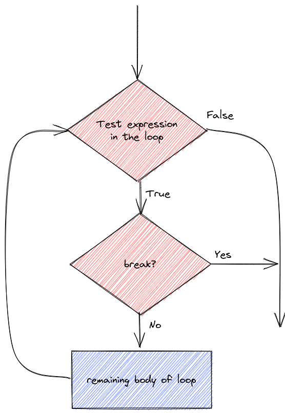
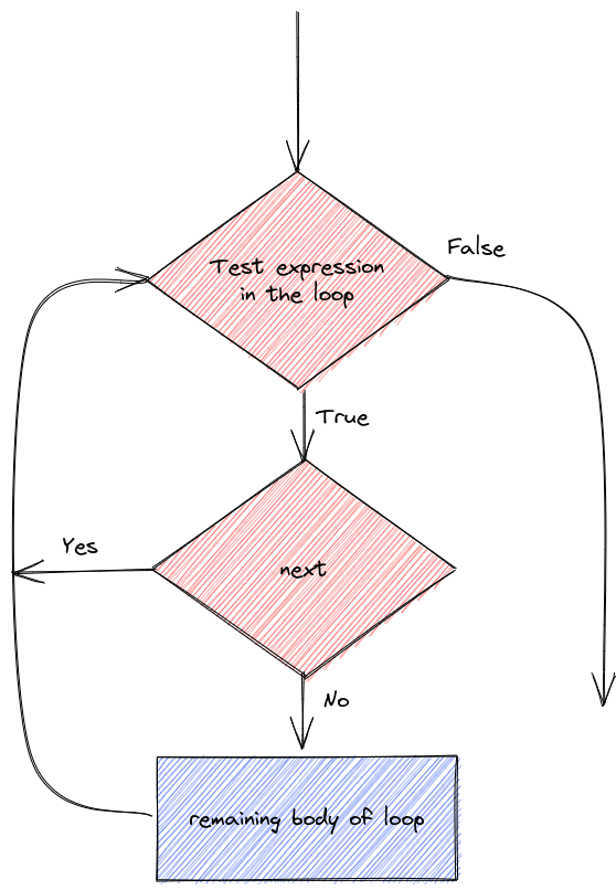
Let’s demonstrate the details of next/continue and break statements.
We can do different things based on whether i is evenly divisible by 3, 5, or both 3 and 5 (thus divisible by 15)
for (i in 1:20) {
  if (i %% 15 == 0) {
    print("Exiting now")
    break
  } else if (i %% 3 == 0) {
    print("Divisible by 3")
    next
    print("After the next statement") # this should never execute
  } else if (i %% 5 == 0) {
    print("Divisible by 5")
  } else {
    print(i)
  }
}
[1] 1
[1] 2
[1] "Divisible by 3"
[1] 4
[1] "Divisible by 5"
[1] "Divisible by 3"
[1] 7
[1] 8
[1] "Divisible by 3"
[1] "Divisible by 5"
[1] 11
[1] "Divisible by 3"
[1] 13
[1] 14
[1] "Exiting now"To be quite honest, I haven’t really ever needed to use next/continue statements when I’m programming, and I rarely use break statements. However, it’s useful to know they exist just in case you come across a problem where you could put either one to use.
This means that doubles take up more memory but can store more decimal places. You don’t need to worry about this much in R.↩︎
In some ways, this is like the difference between an automatic and a manual transmission - you have fewer things to worry about, but you also don’t know what’s going on under the hood nearly as well↩︎
From https://cran.r-project.org/doc/contrib/Short-refcard.pdf↩︎
Throughout this section (and other sections), lego pictures are rendered using https://www.mecabricks.com/en/workshop. It’s a pretty nice tool for building stuff online!↩︎
Grumpy cat, Garfield, Nyan cat. Jorts and Jean: The initial post and the update (both are worth a read because the story is hilarious). The cats also have a Twitter account where they promote workers rights.↩︎