3  Data Cleaning and Manipulation

Reading: 18 minute(s) at 200 WPM.

Videos: 60 minutes

Objectives

• Apply data manipulation verbs (filter, select, group by, summarize, mutate) to prepare data for analysis
• Identify required sequence of steps for data cleaning
• Describe step-by-step data cleaning process in lay terms appropriately and understand the consequences of data cleaning steps
• Create summaries of data appropriate for analysis or display using data manipulation techniques

3.1 A quick note about tibble

We have been talking about our data in terms of data.frame objects in R. This is meant to inform you there is another object type in R called tibbles. Essentially, Tibbles are data frames, but they have certain features that make them easier to work with and provide additional cool features that can be useful (e.g., see nest()).

tibble(
  team   = c("A", "B", "C", "D"), 
  points = c(22, 30, 18, 54)
)

# A tibble: 4 × 2
  team  points
  <chr>  <dbl>
1 A         22
2 B         30
3 C         18
4 D         54

You can use as_tibble() to convert data.frame objects in R to a tibble object.

Learn more about tibbles

You can read more about Tibbles in R for Data Science: Tibbles

3.2 Introduction to dplyr

In this section, we’re going start learning how to work with data. Generally speaking, data doesn’t come in a form suitable for data visualization or statistical analysis¹ - you have to clean it up, create the variables you care about, get rid of those you don’t care about, and so on.

Some people call the process of cleaning and organizing your data “data wrangling”, which is a fantastic way to think about chasing down all of the issues in the data.

Data wrangling (by Allison Horst)

We will be using the tidyverse for this. It’s a meta-package (a package that just loads other packages) that collects packages designed with the same philosophy² and interface (basically, the commands will use predictable argument names and structure). You’ve already been introduced to parts of the tidyverse - specifically, readr and ggplot2.

dplyr (one of the packages in the tidyverse) creates a “grammar of data manipulation” to make it easier to describe different operations. I find the dplyr grammar to be extremely useful when talking about data operations.

Each dplyr verb describes a common task when doing both exploratory data analysis and more formal statistical modeling. In all tidyverse functions, data comes first – literally, as it’s the first argument to any function. In addition, you don’t use df$variable to access a variable - you refer to the variable by its name alone (“bare” names). This makes the syntax much cleaner and easier to read, which is another principle of the tidy philosophy.

Main dplyr verbs

• filter()
• arrange()
• select()
• mutate()
• summarize()
• Use group_by() to perform group wise operations
• Use the pipe operator (|> or %>%) to chain together data wrangling operations

There is an excellent dplyr cheatsheet available from RStudio. You may want to print it out to have a copy to reference as you work through this chapter.

Motivation & Example Dataset

Last week we learned all about creating graphics in ggplot2. I am hoping to use data visualization as motivation going forward in this class – how do we get our data look like what we need in order to create the graph we want?

Let’s explore how the dplyr verbs work, using the starwars data set, which contains a comprehensive list of the characters in the Star Wars movies and information about their height, mass, hair_color, skin_color, eye_color, birth_year, sex, gender, homeworld, species, films, vehicles, and starships.

This data set is included in the dplyr package, so we load that package and then use the data() function to load data set into memory. The loading isn’t complete until we actually use the data set though… so let’s look at our variables and types and print the first few rows.

library(dplyr)
data(starwars)
str(starwars)
starwars

name	height	mass	hair_color	skin_color	eye_color	birth_year	sex	gender	homeworld	species
Luke Skywalker	172	77	blond	fair	blue	19.0	male	masculine	Tatooine	Human
C-3PO	167	75	NA	gold	yellow	112.0	none	masculine	Tatooine	Droid
R2-D2	96	32	NA	white, blue	red	33.0	none	masculine	Naboo	Droid
Darth Vader	202	136	none	white	yellow	41.9	male	masculine	Tatooine	Human
Leia Organa	150	49	brown	light	brown	19.0	female	feminine	Alderaan	Human
Owen Lars	178	120	brown, grey	light	blue	52.0	male	masculine	Tatooine	Human
Beru Whitesun Lars	165	75	brown	light	blue	47.0	female	feminine	Tatooine	Human
R5-D4	97	32	NA	white, red	red	NA	none	masculine	Tatooine	Droid
Biggs Darklighter	183	84	black	light	brown	24.0	male	masculine	Tatooine	Human
Obi-Wan Kenobi	182	77	auburn, white	fair	blue-gray	57.0	male	masculine	Stewjon	Human

We could create a scatterplot of the character’s height by mass, color by species, and facet by homeworld.

library(ggplot2)
ggplot(data = starwars, aes(x = height, 
                            y = mass, 
                            color = species)
       ) +
  geom_point() +
  facet_wrap(~ homeworld)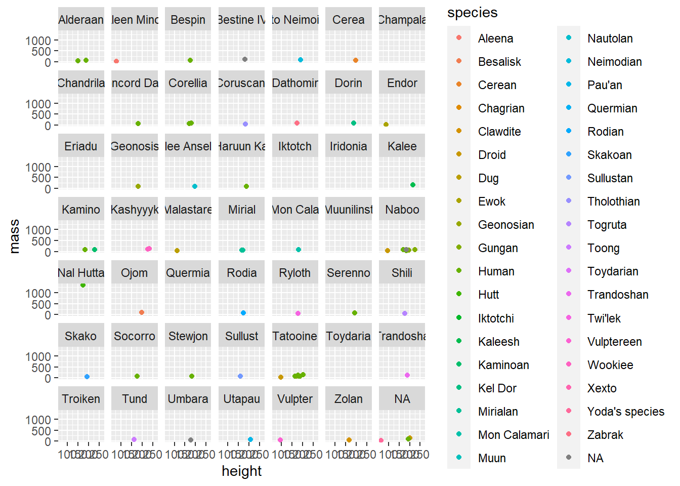

There is way too much going on in these plots to see anything of importance. Let’s break it down into the parts we are interested in.

3.3 filter(): Pick cases (rows) based on their values

Filter allows us to work with a subset of a larger data frame, keeping only the rows we’re interested in. We provide one or more logical conditions, and only those rows which meet the logical conditions are returned from filter(). Note that unless we store the result from filter() in the original object, we don’t change the original.

dplyr filter() by Allison Horst

Once the data is set up, filtering the data (selecting certain rows) is actually very simple. Of course, we’ve talked about how to use logical indexing before in Indexing Matrices, but here we’ll focus on using specific functions to perform the same operation.

The dplyr verb for selecting rows is filter(). filter() takes a set of one or more logical conditions, using bare column names and logical operators. Each provided condition is combined using AND.

Let’s say we were interested in only the people, we could create a new data set starwars_people and filter on the species variable.

# Get only the people
starwars_people <- filter(.data = starwars, 
                          species == "Human"
                          )
starwars_people

name	height	mass	hair_color	skin_color	eye_color	birth_year	sex	gender	homeworld	species
Luke Skywalker	172	77	blond	fair	blue	19.0	male	masculine	Tatooine	Human
Darth Vader	202	136	none	white	yellow	41.9	male	masculine	Tatooine	Human
Leia Organa	150	49	brown	light	brown	19.0	female	feminine	Alderaan	Human
Owen Lars	178	120	brown, grey	light	blue	52.0	male	masculine	Tatooine	Human
Beru Whitesun Lars	165	75	brown	light	blue	47.0	female	feminine	Tatooine	Human

We can create the same plot with our new subset of data (starwars_people).

Code

ggplot(data = starwars_people, 
       mapping = aes(x = height, 
                     y = mass, 
                     color = species
                     )
       ) +
  geom_point() +
  facet_wrap(~ homeworld)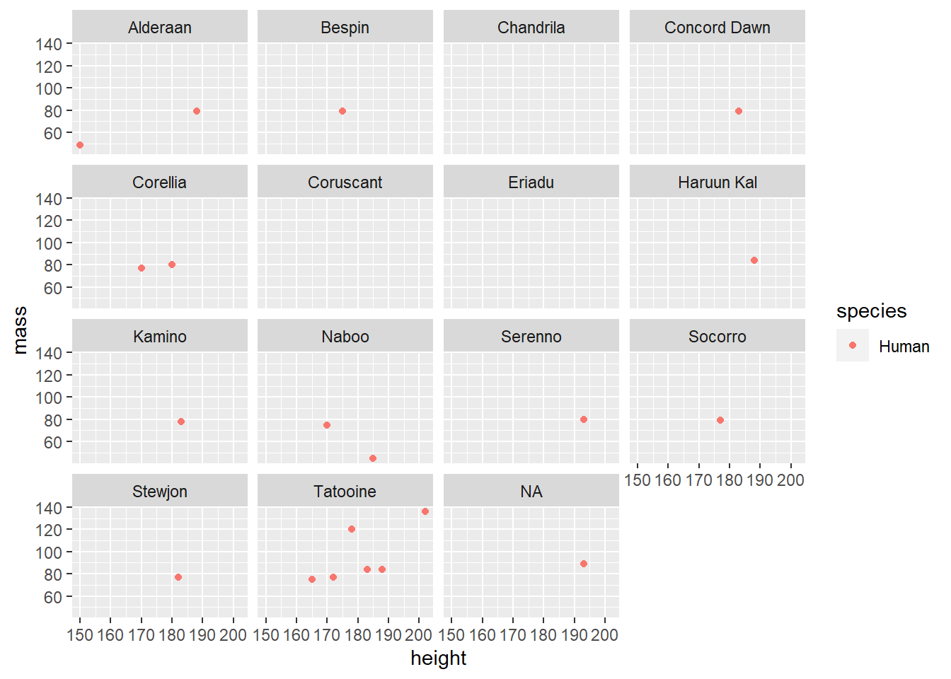

This looks better, but what if we only care about the people who come from Tatooine? Starting with our original starwars data set, we can combine logical AND statements with a comma to define a data subset called starwars_tatoonie_people.

# Get only the people who come from Tatooine
starwars_tatooine_people <- filter(.data = starwars, 
                                   species == "Human", 
                                   homeworld == "Tatooine"
                                   )
starwars_tatooine_people

name	height	mass	hair_color	skin_color	eye_color	birth_year	sex	gender	homeworld	species
Luke Skywalker	172	77	blond	fair	blue	19.0	male	masculine	Tatooine	Human
Darth Vader	202	136	none	white	yellow	41.9	male	masculine	Tatooine	Human
Owen Lars	178	120	brown, grey	light	blue	52.0	male	masculine	Tatooine	Human
Beru Whitesun Lars	165	75	brown	light	blue	47.0	female	feminine	Tatooine	Human
Biggs Darklighter	183	84	black	light	brown	24.0	male	masculine	Tatooine	Human

Code

ggplot(data = starwars_tatooine_people, 
       mapping = aes(x = height, 
                     y = mass, 
                     color = species
                     )
       ) +
  geom_point() +
  facet_wrap(~ homeworld)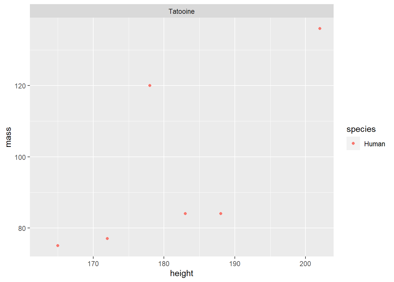

Useful comparison operations in R

We might not always want to only filter on a variable set equal to a certain category or value, the following operations can help you combine logical operations in filter().

• > greater than
• < less than
• == equal to
• %in% identifies if an element belongs to a vector
• | or

3.3.1 Common Row Selection Tasks

In dplyr, there are a few helper functions which may be useful when constructing filter statements.

Filtering by row number

row_number() is a helper function that is only used inside of another dplyr function (e.g. filter). You might want to keep only even rows, or only the first 10 rows in a table.

Notice how we now have C-3PO, Darth Vader, Beru Whites, Anakin Skywalker, etc. (rows 2, 4, 6, …) from the original starwars data set output above.

filter(.data = starwars, 
       row_number() %% 2 == 0
       ) 

Even Rows

name	height	mass	hair_color	skin_color	eye_color	birth_year	sex	gender	homeworld	species
C-3PO	167	75	NA	gold	yellow	112.0	none	masculine	Tatooine	Droid
Darth Vader	202	136	none	white	yellow	41.9	male	masculine	Tatooine	Human
Owen Lars	178	120	brown, grey	light	blue	52.0	male	masculine	Tatooine	Human
R5-D4	97	32	NA	white, red	red	NA	none	masculine	Tatooine	Droid
Obi-Wan Kenobi	182	77	auburn, white	fair	blue-gray	57.0	male	masculine	Stewjon	Human

Original starwars

name	height	mass	hair_color	skin_color	eye_color	birth_year	sex	gender	homeworld	species
Luke Skywalker	172	77	blond	fair	blue	19.0	male	masculine	Tatooine	Human
C-3PO	167	75	NA	gold	yellow	112.0	none	masculine	Tatooine	Droid
R2-D2	96	32	NA	white, blue	red	33.0	none	masculine	Naboo	Droid
Darth Vader	202	136	none	white	yellow	41.9	male	masculine	Tatooine	Human
Leia Organa	150	49	brown	light	brown	19.0	female	feminine	Alderaan	Human
Owen Lars	178	120	brown, grey	light	blue	52.0	male	masculine	Tatooine	Human
Beru Whitesun Lars	165	75	brown	light	blue	47.0	female	feminine	Tatooine	Human
R5-D4	97	32	NA	white, red	red	NA	none	masculine	Tatooine	Droid
Biggs Darklighter	183	84	black	light	brown	24.0	male	masculine	Tatooine	Human
Obi-Wan Kenobi	182	77	auburn, white	fair	blue-gray	57.0	male	masculine	Stewjon	Human

arrange() Sorting rows by variable values

Another common operation is to sort your data frame by the values of one or more variables.

arrange() is a dplyr verb for sorting rows in the table by one or more variables. It is often used with a helper function, desc(), which reverses the order of a variable, sorting it in descending order. Multiple arguments can be passed to arrange to sort the data frame by multiple columns hierarchically; each column can be modified with desc() separately.

The code below arranges the starwars characters tallest to shortest.

arrange(.data = starwars, 
        desc(height)
        )

name	height	mass	hair_color	skin_color	eye_color	birth_year	sex	gender	homeworld	species
Yarael Poof	264	NA	none	white	yellow	NA	male	masculine	Quermia	Quermian
Tarfful	234	136	brown	brown	blue	NA	male	masculine	Kashyyyk	Wookiee
Lama Su	229	88	none	grey	black	NA	male	masculine	Kamino	Kaminoan
Chewbacca	228	112	brown	unknown	blue	200.0	male	masculine	Kashyyyk	Wookiee
Roos Tarpals	224	82	none	grey	orange	NA	male	masculine	Naboo	Gungan
Grievous	216	159	none	brown, white	green, yellow	NA	male	masculine	Kalee	Kaleesh
Taun We	213	NA	none	grey	black	NA	female	feminine	Kamino	Kaminoan
Rugor Nass	206	NA	none	green	orange	NA	male	masculine	Naboo	Gungan
Tion Medon	206	80	none	grey	black	NA	male	masculine	Utapau	Pau'an
Darth Vader	202	136	none	white	yellow	41.9	male	masculine	Tatooine	Human

Keep the top \(n\) values of a variable

slice_max() will keep the top values of a specified variable. This is like a filter statement, but it’s a shortcut built to handle a common task. You could write a filter statement that would do this, but it would take a few more lines of code.

The code below outputs the 5 tallest characters in star wars.

slice_max(.data = starwars, 
          order_by = height, 
          n = 5
          )

name	height	mass	hair_color	skin_color	eye_color	birth_year	sex	gender	homeworld	species
Yarael Poof	264	NA	none	white	yellow	NA	male	masculine	Quermia	Quermian
Tarfful	234	136	brown	brown	blue	NA	male	masculine	Kashyyyk	Wookiee
Lama Su	229	88	none	grey	black	NA	male	masculine	Kamino	Kaminoan
Chewbacca	228	112	brown	unknown	blue	200	male	masculine	Kashyyyk	Wookiee
Roos Tarpals	224	82	none	grey	orange	NA	male	masculine	Naboo	Gungan

Of course, there is a similar slice_min() function as well:

The code below outputs the 5 shortest characters in star wars.

slice_min(.data = starwars, 
          order_by = height, 
          n = 5
          )

name	height	mass	hair_color	skin_color	eye_color	birth_year	sex	gender	homeworld	species
Yoda	66	17	white	green	brown	896	male	masculine	NA	Yoda's species
Ratts Tyerel	79	15	none	grey, blue	unknown	NA	male	masculine	Aleen Minor	Aleena
Wicket Systri Warrick	88	20	brown	brown	brown	8	male	masculine	Endor	Ewok
Dud Bolt	94	45	none	blue, grey	yellow	NA	male	masculine	Vulpter	Vulptereen
R2-D2	96	32	NA	white, blue	red	33	none	masculine	Naboo	Droid
R4-P17	96	NA	none	silver, red	red, blue	NA	none	feminine	NA	Droid

By default, slice_max() and slice_min() return values tied with the nth value as well, which is why our result above has 6 rows.

Use with_ties = FALSE.

slice_min(.data = starwars, 
          order_by = height, 
          n = 5, 
          with_ties = FALSE
          )

name	height	mass	hair_color	skin_color	eye_color	birth_year	sex	gender	homeworld	species
Yoda	66	17	white	green	brown	896	male	masculine	NA	Yoda's species
Ratts Tyerel	79	15	none	grey, blue	unknown	NA	male	masculine	Aleen Minor	Aleena
Wicket Systri Warrick	88	20	brown	brown	brown	8	male	masculine	Endor	Ewok
Dud Bolt	94	45	none	blue, grey	yellow	NA	male	masculine	Vulpter	Vulptereen
R2-D2	96	32	NA	white, blue	red	33	none	masculine	Naboo	Droid

slice_max and slice_min also take a prop argument that gives you a certain proportion of the values:

The code below outputs the shortest 1% of characters in star wars.

slice_max(.data = starwars, 
          order_by = height, 
          prop = 0.01
          )

name	height	mass	hair_color	skin_color	eye_color	birth_year	sex	gender	homeworld	species

3.4 select(): Pick columns

Sometimes, we don’t want to work with a set of 50 variables when we’re only interested in 5. When that happens, we might be able to pick the variables we want by index (e.g. df[, c(1, 3, 5)]), but this can get tedious.

In dplyr, the function to pick a few columns is select(). The syntax from the help file (?select) looks deceptively simple.

select(.data, …)

So as with just about every other tidyverse function, the first argument in a select statement is the data (.data =). After that, though, you can put just about anything that R can interpret. ... means something along the lines of “put in any additional arguments that make sense in context or might be passed on to other functions”.

So what can go in there?

An exhaustive(?) list of ways to select variables in dplyr

First, dplyr aims to work with standard R syntax, making it intuitive (and also, making it work with variable names instead of just variable indices).³
Most dplyr commands work with “bare” variable names - you don’t need to put the variable name in quotes to reference it. There are a few exceptions to this rule, but they’re very explicitly exceptions.

• var3:var5: select(df, var3:var5) will give you a data frame with columns var3, anything between var3 and var 5, and var5

• !(<set of variables>) will give you any columns that aren’t in the set of variables in parentheses

  • (<set of vars 1>) & (<set of vars 2>) will give you any variables that are in both set 1 and set 2. (<set of vars 1>) | (<set of vars 2>) will give you any variables that are in either set 1 or set 2.
  • c() combines sets of variables.

dplyr also defines a lot of variable selection “helpers” that can be used inside select() statements. These statements work with bare column names (so you don’t have to put quotes around the column names when you use them).

• everything() matches all variables
• last_col() matches the last variable. last_col(offset = n) selects the n-th to last variable.
• starts_with("xyz") will match any columns with names that start with xyz. Similarly, ends_with() does exactly what you’d expect as well.
• contains("xyz") will match any columns with names containing the literal string “xyz”. Note, contains does not work with regular expressions (you don’t need to know what that means right now).
• matches(regex) takes a regular expression as an argument and returns all columns matching that expression.
• num_range(prefix, range) selects any columns that start with prefix and have numbers matching the provided numerical range.

There are also selectors that deal with character vectors. These can be useful if you have a list of important variables and want to just keep those variables.

• all_of(char) matches all variable names in the character vector char. If one of the variables doesn’t exist, this will return an error.
• any_of(char) matches the contents of the character vector char, but does not throw an error if the variable doesn’t exist in the data set.

There’s one final selector -

• where() applies a function to each variable and selects those for which the function returns TRUE. This provides a lot of flexibility and opportunity to be creative.

Let’s try these selector functions out and see what we can accomplish!

Starting simple, let’s only subset and keep only the following variables from the starwars data set: name, height, mass, birth_year, species, and homeworld.

select(.data = starwars, name, height, mass, birth_year, species, homeworld)

name	height	mass	birth_year	species	homeworld
Luke Skywalker	172	77	19.0	Human	Tatooine
C-3PO	167	75	112.0	Droid	Tatooine
R2-D2	96	32	33.0	Droid	Naboo
Darth Vader	202	136	41.9	Human	Tatooine
Leia Organa	150	49	19.0	Human	Alderaan
Owen Lars	178	120	52.0	Human	Tatooine
Beru Whitesun Lars	165	75	47.0	Human	Tatooine
R5-D4	97	32	NA	Droid	Tatooine
Biggs Darklighter	183	84	24.0	Human	Tatooine
Obi-Wan Kenobi	182	77	57.0	Human	Stewjon

Since name, height, and mass are next to each other, we could have specified name:mass to tell us to select all of the columns between and including name to mass.

select(.data = starwars, name:mass, birth_year, species, homeworld)

name	height	mass	birth_year	species	homeworld
Luke Skywalker	172	77	19.0	Human	Tatooine
C-3PO	167	75	112.0	Droid	Tatooine
R2-D2	96	32	33.0	Droid	Naboo
Darth Vader	202	136	41.9	Human	Tatooine
Leia Organa	150	49	19.0	Human	Alderaan
Owen Lars	178	120	52.0	Human	Tatooine
Beru Whitesun Lars	165	75	47.0	Human	Tatooine
R5-D4	97	32	NA	Droid	Tatooine
Biggs Darklighter	183	84	24.0	Human	Tatooine
Obi-Wan Kenobi	182	77	57.0	Human	Stewjon

The select column is also useful for reordering the variables in your data set.

:::

Perhaps we want the birth_year, sex, gender, homeworld, and species to follow the name of the star wars character. We can use the everything() function to specify we want all the other variables to follow.

select(.data = starwars, name, birth_year:species, everything())

name	birth_year	sex	gender	homeworld	species	height	mass	hair_color	skin_color	eye_color
Luke Skywalker	19.0	male	masculine	Tatooine	Human	172	77	blond	fair	blue
C-3PO	112.0	none	masculine	Tatooine	Droid	167	75	NA	gold	yellow
R2-D2	33.0	none	masculine	Naboo	Droid	96	32	NA	white, blue	red
Darth Vader	41.9	male	masculine	Tatooine	Human	202	136	none	white	yellow
Leia Organa	19.0	female	feminine	Alderaan	Human	150	49	brown	light	brown
Owen Lars	52.0	male	masculine	Tatooine	Human	178	120	brown, grey	light	blue
Beru Whitesun Lars	47.0	female	feminine	Tatooine	Human	165	75	brown	light	blue
R5-D4	NA	none	masculine	Tatooine	Droid	97	32	NA	white, red	red
Biggs Darklighter	24.0	male	masculine	Tatooine	Human	183	84	black	light	brown
Obi-Wan Kenobi	57.0	male	masculine	Stewjon	Human	182	77	auburn, white	fair	blue-gray

Note that everything() won’t duplicate columns you’ve already added.

:::

So for now, at least in R, you know how to cut your data down to size rowwise (with filter) and column-wise (with select).

dplyr::relocate

Another handy dplyr function is relocate; while you definitely can do this operation in many, many different ways, it may be simpler to do it using relocate. But, I’m covering relocate here mostly because it also comes with this amazing cartoon illustration.

relocate lets you rearrange columns (by Allison Horst)

# move numeric variables to the front
relocate(.data = starwars, 
         where(is.numeric)
         )

# A tibble: 87 × 11
   height  mass birth_year name     hair_color skin_color eye_color sex   gender
    <int> <dbl>      <dbl> <chr>    <chr>      <chr>      <chr>     <chr> <chr> 
 1    172    77       19   Luke Sk… blond      fair       blue      male  mascu…
 2    167    75      112   C-3PO    <NA>       gold       yellow    none  mascu…
 3     96    32       33   R2-D2    <NA>       white, bl… red       none  mascu…
 4    202   136       41.9 Darth V… none       white      yellow    male  mascu…
 5    150    49       19   Leia Or… brown      light      brown     fema… femin…
 6    178   120       52   Owen La… brown, gr… light      blue      male  mascu…
 7    165    75       47   Beru Wh… brown      light      blue      fema… femin…
 8     97    32       NA   R5-D4    <NA>       white, red red       none  mascu…
 9    183    84       24   Biggs D… black      light      brown     male  mascu…
10    182    77       57   Obi-Wan… auburn, w… fair       blue-gray male  mascu…
# ℹ 77 more rows
# ℹ 2 more variables: homeworld <chr>, species <chr>

3.5 mutate(): Add and transform variables

Up to this point, we’ve been primarily focusing on how to decrease the dimensionality of our data set in various ways (i.e., remove rows or columns from the original data set). But frequently, we also need to add columns for derived measures (e.g. BMI from weight and height information), change units, and replace missing or erroneous observations. The tidyverse verb for this is mutate().

Mutate (by Allison Horst)

Let’s create a new variable, BMI calculated from existing columns – mass/height\(^2\)

mutate(.data = starwars, 
       BMI = mass/height^2, 
       .after = mass
       )

name	height	mass	BMI	hair_color	skin_color	eye_color	birth_year	sex	gender	homeworld	species
Luke Skywalker	172	77	0.0026028	blond	fair	blue	19.0	male	masculine	Tatooine	Human
C-3PO	167	75	0.0026892	NA	gold	yellow	112.0	none	masculine	Tatooine	Droid
R2-D2	96	32	0.0034722	NA	white, blue	red	33.0	none	masculine	Naboo	Droid
Darth Vader	202	136	0.0033330	none	white	yellow	41.9	male	masculine	Tatooine	Human
Leia Organa	150	49	0.0021778	brown	light	brown	19.0	female	feminine	Alderaan	Human
Owen Lars	178	120	0.0037874	brown, grey	light	blue	52.0	male	masculine	Tatooine	Human
Beru Whitesun Lars	165	75	0.0027548	brown	light	blue	47.0	female	feminine	Tatooine	Human
R5-D4	97	32	0.0034010	NA	white, red	red	NA	none	masculine	Tatooine	Droid
Biggs Darklighter	183	84	0.0025083	black	light	brown	24.0	male	masculine	Tatooine	Human
Obi-Wan Kenobi	182	77	0.0023246	auburn, white	fair	blue-gray	57.0	male	masculine	Stewjon	Human

By default, the new variable will be tacked on to the end of the data set as the last column. Using .after or .before arguments allows you to place the new variable in the middle of the data set.

We can combine the mutate function with other variables such as ifelse().

Let’s replace the species variable to indicate Human or Not Human.

mutate(.data = starwars, 
       species = if_else(species == "Human", 
                        species, 
                        "Not Human"
                        )
       )

name	height	mass	hair_color	skin_color	eye_color	birth_year	sex	gender	homeworld	species
Luke Skywalker	172	77	blond	fair	blue	19.0	male	masculine	Tatooine	Human
C-3PO	167	75	NA	gold	yellow	112.0	none	masculine	Tatooine	Not Human
R2-D2	96	32	NA	white, blue	red	33.0	none	masculine	Naboo	Not Human
Darth Vader	202	136	none	white	yellow	41.9	male	masculine	Tatooine	Human
Leia Organa	150	49	brown	light	brown	19.0	female	feminine	Alderaan	Human
Owen Lars	178	120	brown, grey	light	blue	52.0	male	masculine	Tatooine	Human
Beru Whitesun Lars	165	75	brown	light	blue	47.0	female	feminine	Tatooine	Human
R5-D4	97	32	NA	white, red	red	NA	none	masculine	Tatooine	Not Human
Biggs Darklighter	183	84	black	light	brown	24.0	male	masculine	Tatooine	Human
Obi-Wan Kenobi	182	77	auburn, white	fair	blue-gray	57.0	male	masculine	Stewjon	Human

The learning curve here isn’t actually knowing how to assign new variables (though that’s important). The challenge comes when you want to do something new and have to figure out how to e.g. use find and replace in a string, or work with dates and times, or recode variables. We will cover special data types like these in a few weeks!

Mutate and new challenges

I’m not going to be able to teach you how to handle every mutate statement task you’ll come across (people invent new ways to screw up data all the time!) but my goal is instead to teach you how to read documentation and Google things intelligently, and to understand what you’re reading enough to actually implement it. This is something that comes with practice (and lots of Googling, stack overflow searches, etc.).

Google and StackOverflow are very common and important programming skills!

Source

Source

In this textbook, the examples will expose you to solutions to common problems (or require that you do some basic reading yourself); unfortunately, there are too many common problems for us to work through line-by-line.

Part of the goal of this textbook is to help you learn how to read through a package description and evaluate whether the package will do what you want. We’re going to try to build some of those skills starting now. It would be relatively easy to teach you how to do a set list of tasks, but you’ll be better statisticians and programmers if you learn the skills to solve niche problems on your own.

Apologies for the noninclusive language, but the sentiment is real. Source

3.6 summarize()

The next verb is one that we’ve already implicitly seen in action: summarize() takes a data frame with potentially many rows of data and reduces it down to one row of data using some function.

Here (in a trivial example), I compute the overall average height of a star war’s character.

summarize(.data = starwars,
          avg_height = mean(height, na.rm = T)
          )

# A tibble: 1 × 1
  avg_height
       <dbl>
1       175.

The na.rm = T argument says to ignore/remove the missing (NA) values in calculating the average.

The real power of summarize, though, is in combination with group_by. We’ll see more summarize examples, but it’s easier to make good examples when you have all the tools - it’s hard to demonstrate how to use a hammer if you don’t also have a nail.

3.7 group_by() Group By + (?) = Power!

Frequently, we have data that is more specific than the data we need - for instance, I may have observations of the temperature at 15-minute intervals, but I might want to record the daily high and low value. To do this, I need to

1. split my data set into smaller data sets - one for each day
2. compute summary values for each smaller data set
3. put my summarized data back together into a single data set

This is known as the split-apply-combine “Group by: Split-Apply-Combine” (2022) or sometimes, map-reduce (Dean and Ghemawat 2008) strategy (though map-reduce is usually on specifically large data sets and performed in parallel).

In tidy parlance, group_by() is the verb that accomplishes the first task. summarize() accomplishes the second task and implicitly accomplishes the third as well.

Let’s see how things change when we calculate the average height of star wars characters by their species.

starwars |> 
  group_by(species) |> 
  summarize(height = mean(height, na.rm = T))

# A tibble: 38 × 2
   species   height
   <chr>      <dbl>
 1 Aleena       79 
 2 Besalisk    198 
 3 Cerean      198 
 4 Chagrian    196 
 5 Clawdite    168 
 6 Droid       131.
 7 Dug         112 
 8 Ewok         88 
 9 Geonosian   183 
10 Gungan      209.
# ℹ 28 more rows

The next section Pipe Operator will introduce and talk about what the |> symbol is, this example is just hard to show without it!

The ungroup() command is just as important as the group_by() command! (by Allison Horst)

When you group_by() a variable, your result carries this grouping with it. summarize() will remove one layer of grouping (by default), but if you ever want to return to a completely ungrouped data set, you should use the ungroup() command.

3.8 Pipe Operator

The powerhouse of the tidyverse package comes from the pipe operator. This specifies a sequence of operations (kind of like how we layered our graphics in ggplot2). The output from the previous line (often a subset) is automatically passed into the first argument of the next line (remember, data first! .data =).

The native pipe operator is |>, but the magrittr pipe operator %>% was used up until recently (and still is often used!).

The keyboard shortcut for adding a pipe operator to your code is Ctrl/Cmd + Shift + M.

However, if you want to use this shortcut for the native pipe, you need to change your global R settings:

Tools > Global Options > Code > checkbox Use native pipe operator, |>

(required) Read more about the pipe operators at Workflow Pipes and Formatting Pipes.

Let’s combine all of our new skills with the pipe operator!

1. Use filter() to subset our data to only Human’s and Droid’s
2. Use mutate() to create the new variable, BMI,
3. Use group_by() to create groups by species,
4. Use summarize() to calculate the mean and standard deviation of BMI
5. Use mutate() to calculate the average plus/minus one standard deviation.

We could either assign this new data set that has summary values of BMI by species or we could pipe the data set directly into a plot – recall the first argument for ggplot() is data =.

starwars |> 
  filter(species %in% c("Human", "Droid")) |> 
  mutate(BMI = mass/height^2) |> 
  group_by(species) |> 
  summarize(avg_BMI = mean(BMI, na.rm = TRUE),
            sd_BMI = sd(BMI, na.rm = TRUE)
            ) |> 
  mutate(BMI_1sd_below = avg_BMI - sd_BMI,
         BMI_1sd_above = avg_BMI + sd_BMI
         ) |> 
  ggplot(aes(x = species, 
             y = avg_BMI)
         ) +
  geom_point() +
  geom_errorbar(aes(ymin = BMI_1sd_below,
                    ymax = BMI_1sd_above),
                width = 0.2
                ) +
  labs(x = "Species", 
       subtitle = "Average BMI") +
  theme(axis.title.y = element_blank())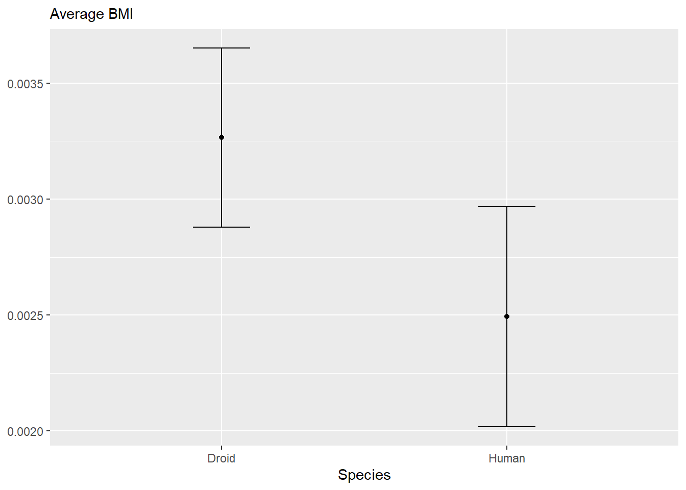

As with ggplot, formatting your dplyr code pipelines so it is readable will help both you and me!

Additional Resources

• Introduction to dplyr and Single Table dplyr functions

• R for Data Science: Data Transformations

• Modern Dive: Data Wrangling

• Additional practice exercises: Intro to the tidyverse, group_by + summarize examples, group_by + mutate examples (from a similar class at Iowa State)

• Videos of analysis of new data from Tidy Tuesday - may include use of other packages, but almost definitely includes use of dplyr as well.

References

Dean, Jeffrey, and Sanjay Ghemawat. 2008. “MapReduce: Simplified Data Processing on Large Clusters.” Communications of the ACM 51 (1): 107–13. https://doi.org/10.1145/1327452.1327492.

“Group by: Split-Apply-Combine.” 2022. In Pandas 1.4.3 Documentation. Python. https://pandas.pydata.org/pandas-docs/stable/user_guide/groupby.html.

Wickham, Hadley. 2011. “The Split-Apply-Combine Strategy for Data Analysis.” Journal of Statistical Software 40: 1–29.

---

1. See this twitter thread for some horror stories. This tweet is also pretty good at showing one type of messiness.

2. The philosophy includes a preference for pipes, but this preference stems from the belief that code should be readable in the same way that text is readable.

3. It accomplishes this through the magic of quasiquotation, which we will not cover in this course because it’s basically witchcraft.